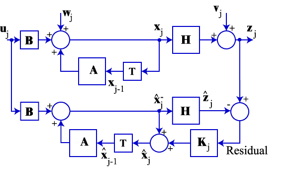
The matrix problem proceeds just as the scalar problem, but all of the variables are now matrices. The system has p inputs, n state variables and m outputs.
| variable | Scalar | Matrix | Matrix size |
| state | xj | xj | n by 1 |
| input | uj | uj | p by 1 |
| output | zj | zj | m by 1 |
| state gain | a | A | n by n |
| input gain | b | B | n by p |
| output gain | h | Hj | m by n |
| process noise | wj | wj | n by 1 |
| process noise covariance | Q | Q | n by n |
| measurement noise | vj | vj | m by 1 |
| measurement noise covariance | R | R | m by m |
| a priori covariance | n by n | ||
| a posteriori covariance | n by n | ||
| Kalman Filter Gain | kj | Kj | n by m |
The solution proceeds as did the scalar case. Only major results will be presented here, the intermediate results are not discussed, but can be determined by analogy with the derivation of the scalar kalman filter.
A discrete time system with process noise w and measurement noise v is defined by:
Equation 1
The corresponding block diagram is shown below


 Equation 4