You are given the transfer function of a system as
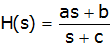 . Answer parts a-d without performing an inverse Laplace Transform.
a) What is the time constant associated with the system? (Remember that the homogeneous response can be written in terms of the time constant in the form e-t/τ; what are the form of the exponential response due to H(s) (you may consult a Laplace Transform table to answer)).
b) What is the final value of the unit step response.
c) What is the initial value, at t=0+, of the unit step response.
d) The step response of a first order system is given by
 .
Use your results from parts a-c to write an expression for the unit step response.
e) Find the unit step response of the system defined by H(s), given above, using the inverse Laplace Transform.
a) Solutions will have exponentials of the form e-ct. Therefore τ=1/c.
b)

c)

d) 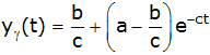
e) 
The graph below
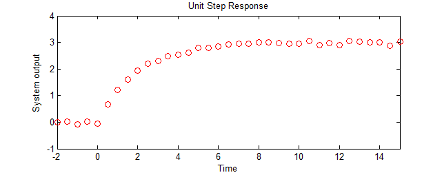
shows experimental data for a system with unit step applied at t=0 (and initial condition=0 at t=0-). The response of a system and can be described by the equation (for t≥0).

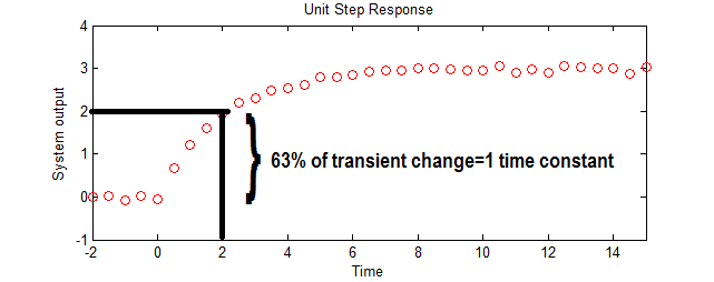
a) What are approximate values for A and τ (rounded to the nearest integer).
b) What is the Laplace Transform of the step response?
c) Express the transfer function as a ratio of polynomials?
d) What is the differential equation that describes the system (input=f(t), output=y(t))?
a) A=3, τ=2, α=0.5;
b) 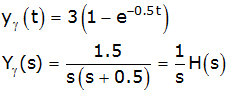
c)
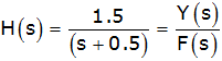
d)

The principles of linear constant coefficient differential equations can be applied to many physiological systems. One straightforward application is compartmental analysis.
The next 3 paragraphs are for background only, you can easily skip them and just work with the equations.
The main assumption of this technique is that the body is made up of many compartments. Drugs, or other substances, move out of source compartments into one or more destination compartments at a rate proportional to the concentration of drugs in the source compartment. Each destination compartment has its own rate constant. We will consider a very simple case with only two compartments, and drug flow only in one direction (in the general case, flow can be bi-directional with a different rate constant in each direction).
Consider the metabolism of alcohol, and assume a two-compartment model.
Alcohol is ingested into the first compartment, the gastro-intestinal (or GI
-- this consists of your stomach, intestines…) tract. Alcohol moves out
of the GI to the second compartment, the blood, at a rate that is dependent
on the concentration of blood in the GI tract. Alcohol leaving the GI
tract enters the blood, and alcohol leaves the blood (through metabolism and
excretion) at a rate proportional to the concentration of alcohol in the blood.
The quantities in the system are given by:
- i(t) is alcohol consumption
- g(t) is the concentration of alcohol in the GI tract.
- c(t) is the concentration of alcohol in the blood.
- k0 is the rate constant for alcohol leaving the GI tract and entering the blood.
- k1 is the rate constant for alcohol leaving the blood.
A block diagram is shown below:

We can write differential equations for the GI concentration. g(t) and the blood concentration c(t):
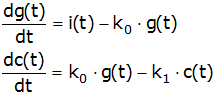
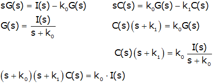
a) Verify that, for the zero-state case (no initial conditions) that:

Show all steps involved in your response.
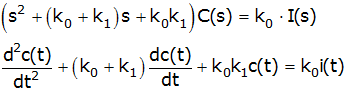
b) What is the differential equation relating c(t) and i(t)?
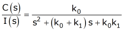
c) What is the transfer function (the ratio of output to input) H(s)=C(s)/I(s)?
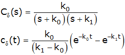
d) Find the imputse response, h(t). In other words find c(t) if i(t)=δ(t). This corresponds to a single dose of alcohol, ingested quickly. Show all steps involved in your response. Note the units of c(t) are aribitrary, and not Blood Acohol Content as is usually measured. But the dynamics (speed) of the equations are correct.
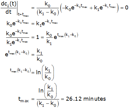
e) Use your expression for c(t) from above to find the time at which alcohol concentration in the blood is at a maximum. What does this suggest about the time at which you are most impaired after a drink.
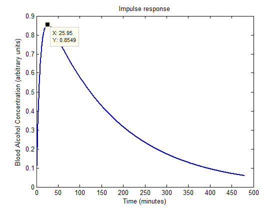
f) Make and print an accurate plot of c(t). Check the peak time against your previous calculation. Include any Matlab code (well commented).
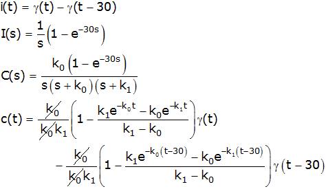
g) If you drink steadily for 1/2 hour (i.e., the function i(t) is a rectangular pulse of amplitude 1 and width 30 minutes), write an expression for i(t), I(s), C(s) and c(t). Plot c(t). Include any Matlab code (well commented).
a)
b)
c)
d)
e) Peak at
f)
t=linspace(0,480,1000);  % Six hours
c_delta=k0*(exp(-k0*t)-exp(-k1*t))/(k1-k0);  % Impulse response
plot(t,c_delta,'Linewidth',2);  %Plot
xlabel('Time (minutes)')'
ylabel('Blood Alcohol Concentration (arbitrary units)');
title('Impulse response');
tmax=t(c_delta==max(c_delta))  % Display time of maximum
g)
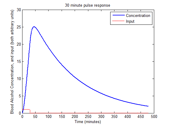
t=linspace(0,480,1000);  % Six hours
c=(1-(k1*exp(-k0*t)-k0*exp(-k1*t))/(k1-k0))/k1.*(t>=0)-...   % Pulse response
    (1-(k1*exp(-k0*(t-30))-k0*exp(-k1*(t-30)))/(k1-k0))/k1.*(t>=30);
plot(t,c,'b','Linewidth',2);  %Plot concentration
hold on;
plot(t,(t>=0)-(t>=30),'r:','Linewidth',2);  %Plot input
hold off;
legend('Concentration','Input');
xlabel('Time (minutes)');
ylabel('Blood Alcohol Concentration, and input (both arbitrary units)');
title('30 minute pulse response');
tmax=t(c_delta==max(c_delta))  % Display time of maximum
Consider the system shown below (the unlabeled friction is "b"). A student (but maybe not an A student) gets the free body diagram incorrect, as shown.
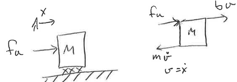
a) Using the incorrect free body diagram, find an expression for and sketch the impulse response (the sketch is necessarily crude since no numbers are given). Also sketch a pole-zero diagram
b) Explain the shape of the graph.
c) Draw the correct free body diagram and repeat a and b.
Solution

For the three circuits shown:
| Circuit i | 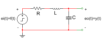 |
| Circuit ii | 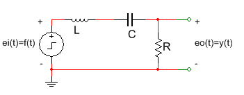 |
| Circuit iii | 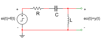 |
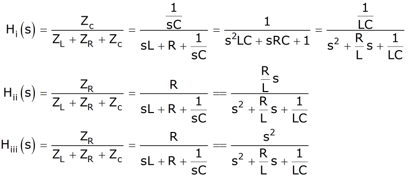
a) Write the three transfer function Hi(s), Hii(s) and Hiii(s) (input=f(t)=ei(t), output=y(t)=eo(t)). You can find the transfer function using the voltage divider equation with ZC=1/(sC), ZL=sL, and ZR=R.
For the next parts assume the input is a unit step (f(t)=γ(t)) and initial conditions at t=0- are all zero. Also assume that the system is overdamped so there are no oscillations.
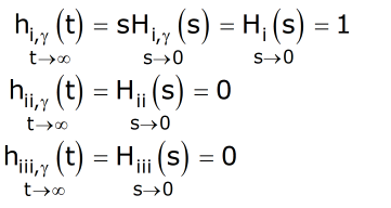
b) Find the output of each system as t→∞. Use the final value theorem. This should agree with what you know about the behavior of circuit components at t→∞ for a constant input.
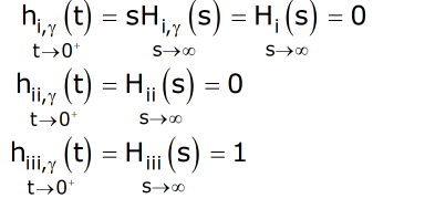
c) Find initial conditions on y(t) at t=0+. Use the inital value theorem.
d) Very crudely sketch the step response for an overdamped system. Pay particular attention to the response for t near 0 and ∞. Note there are no actual numbers so you can't sketch with any accuracy, and you'll have to make an educated guess about the slope at t=0+.
e) Answer the following questions. Based on the order of the derivative of the input (i.e., the power of "s" in the numerator).
- ...what can you say about the steady state value of the output as t→∞?
- ...what can you say about the nature of any discontinuities of the system between t=0- and t=0+.
a)
b)
c)
d) Note each output looks like the derivative of the one that precedes it.
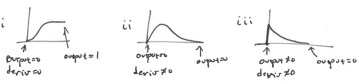
e) If there is any derivative of the input, the output goes to zero as t→∞. If the order of the derivative on the right side is the same as the order of the highest derivative on the left side, then there is a discontinuity of the output between t=0- and t=0+. (Note: I don't expect you to generalize (yet), but as the order of the derivative on the RHS increases, the output undergoes more drastic changes from t=0- to t=0+.)
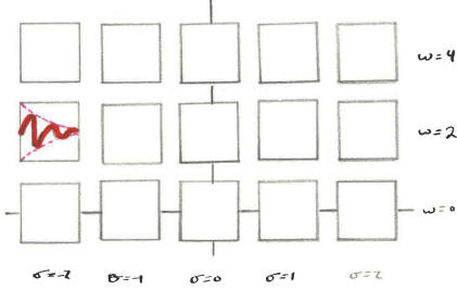
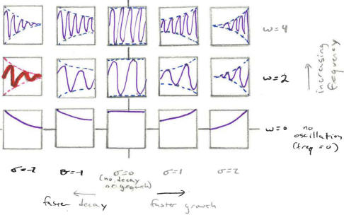
The plot below represents the Laplace plane (i.e., the variable s). The horizontal axis is the real part of s, the vertical axis is the imaginary part such that s=σ+jω. If the poles of a transfer function existed at the center of a square, sketch the corresponding response in the square (for complex values of s, assume that there is a corresponding complex conjugate pole). For the square that is already filled in σ=-2 and ω=2. This square shows a decreasing function due to a response of the form e(σ+jω)t (plus a corresponding conjugate term). Clearly indicate similarities and differences in the expected responses corresponding to differences in σ and ω. You don't need to try to figure things out in terms of ζ and ω0.